Trees and Graphs

Readings

Binary tree

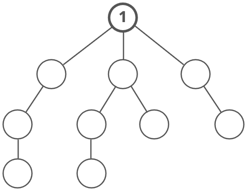
A binary tree is a tree where every node has two or fewer children. The children are usually called left and right.

class BinaryTreeNode {
  constructor(value) {
    this.value = value;
    this.left  = null;
    this.right = null;
  }
}

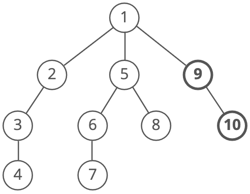
This lets us build a structure like this:

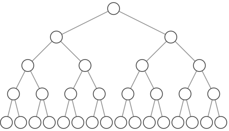
That particular example is special because every level of the tree is completely full. There are no "gaps." We call this kind of tree "perfect." Binary trees have a few interesting properties when they're perfect:

Property 1: The number of total nodes on each "level" doubles as we move down the tree.

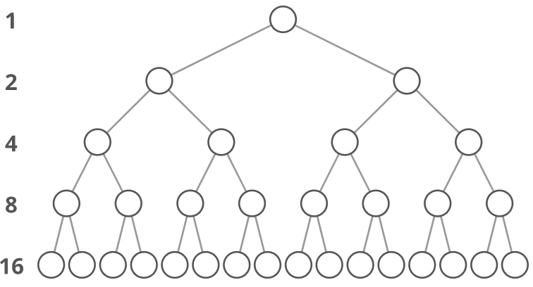
Property 2: The number of nodes on the last level is equal to the sum of the number of nodes on all other levels (plus 1).

In other words, about half of our nodes are on the last level. Let's call the number of nodes $n$, and the height of the tree $h$. $h$ can also be thought of as the "number of levels." If we had $h$, how could we calculate $n$? Let's just add up the number of nodes on each level. How many nodes are on each level? If we zero-index the levels, the number of nodes on the $x$th level is exactly $2^x$.

1. Level 0: $2^0$ nodes,
2. Level 1: $2^1$ nodes,
3. Level 2: $2^2$ nodes,
4. Level 3: $2^3$ nodes,
5. etc.

So our total number of nodes is:

$$n=2^0+2^1+2^2+2^3+\cdots+2^{h-1}$$

Why only up to $2^{h-1}$? Notice that we started counting our levels at 0. So if we have $h$ levels in total, the last level is actually the "$h-1$"-th level. That means the number of nodes on the last level is $2^{h-1}$.

But we can simplify. Property 2 tells us that the number of nodes on the last level is (1 more than) half of the total number of nodes, so we can just take the number of nodes on the last level, multiply it by 2, and subtract 1 to get the number of nodes overall. We know the number of nodes on the last level is $2^{h-1}$, so:

$$\begin{align*} n&= 2^{h-1}\cdot2 - 1\newline n&= 2^{h-1}\cdot2^1 - 1\newline n&= 2^{h-1+1} - 1\newline n&= 2^h - 1\newline \end{align*}$$

So that's how we can go from $h$ to $n$. What about the other direction? We need to bring the $h$ down from the exponent. That's what logs are for! First, some quick review. $\log_{10}100$ simply means, "What power must you raise 10 to in order to get 100?" Which is 2, because $10^2=100$. We can use logs in algebra to bring variables down from exponents by exploiting the fact that we can simplify $\log_{10}100$. What power must we raise 10 to in order to get $10^2$? That's easy--it's 2.

So in this case we can take the $\log_2$ of both sides:

$$\begin{align*} n&=2^h-1\newline n+1&=2^h\newline \log_2(n+1)&=\log_2(2^h)\newline \log_2(n+1)&=h \end{align*}$$

So that's the relationship between height and total nodes in a perfect binary tree.

Graph

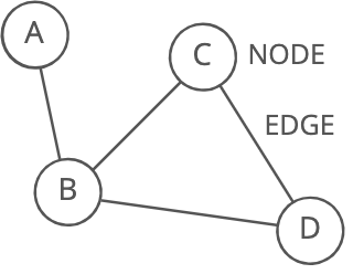
Description: Good for storing networks, geography, social relationships, etc. A graph organizes items in an interconnected network. Each item is a node (or vertex). Nodes are connected by edges:

Visual description:

Strengths:

• Representing links: Graphs are ideal for cases where you're working with things that connect to other things. Nodes and edges could, for example, respectively represent cities and highways, routers and ethernet cables, or Facebook users and their friendships.

Weaknesses:

• Scaling challenges: Most graph algorithms are $O(n\lg n)$ or even slower. Depending on the size of your graph, running algorithms across your nodes may not be feasible.

Terminology

Directed or undirected: In directed graphs, edges point from the node at one end to the node at the other end. In undirected graphs, the edges simply connect the nodes at each end.

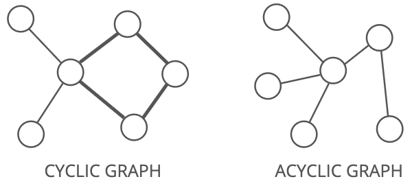
Cyclic or acyclic: A graph is cyclic if it has a cycle—-an unbroken series of nodes with no repeating nodes or edges that connects back to itself. Graphs without cycles are acyclic.

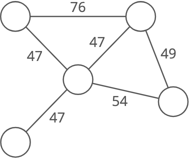
Weighted or unweighted: If a graph is weighted, each edge has a "weight." The weight could, for example, represent the distance between two locations, or the cost or time it takes to travel between the locations.

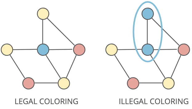
Legal coloring: A graph coloring is when you assign colors to each node in a graph. A legal coloring means no adjacent nodes have the same color:

Representations

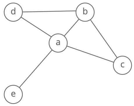
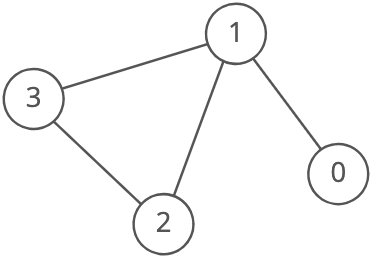
There are a few different ways to store graphs. Let's take this graph as an example:

Edge list

A list of all the edges in the graph:

const graph = [[0, 1], [1, 2], [1, 3], [2, 3]];

Since node 3 has edges to nodes 1 and 2, [1, 3] and [2, 3] are in the edge list.

Sometimes it's helpful to pair our edge list with a list of all the nodes. For example, what if a node doesn't have any edges connected to it? It wouldn't show up in our edge list at all!

Adjacency list

A list where the index represents the node and the value at that index is a list of the node's neighbors:

const graph = [
  [1],
  [0, 2, 3],
  [1, 3],
  [1, 2],
];

Since node 3 has edges to nodes 1 and 2, graph[3] has the adjacency list [1, 2].

We could also use an object where the keys represent the node and the values are the lists of neighbors.

const graph = {
  0: [1],
  1: [0, 2, 3],
  2: [1, 3],
  3: [1, 2],
};

This would be useful if the nodes were represented by strings, objects, or otherwise didn't map cleanly to array indices.

Adjacency matrix

A matrix of 0s and 1s indicating whether node x connects to node y (0 means no, 1 means yes).

const graph = [
  [0, 1, 0, 0],
  [1, 0, 1, 1],
  [0, 1, 0, 1],
  [0, 1, 1, 0],
];

Since node 3 has edges to nodes 1 and 2, graph[3][1] and graph[3][2] have value 1.

Algorithms

BFS and DFS

You should know breadth-first search (BFS) and depth-first search (DFS) down pat so you can code them up quickly. Lots of graph problems can be solved using just these traversals:

• Is there a path between two nodes in this undirected graph? Run DFS or BFS from one node and see if you reach the other one.
• What's the shortest path between two nodes in this undirected, unweighted graph? Run BFS from one node and backtrack once you reach the second. Note: BFS always finds the shortest path, assuming the graph is undirected and unweighted. DFS does not always find the shortest path.
• Can this undirected graph be colored with two colors? Run BFS, assigning colors as nodes are visited. Abort if we ever try to assign a node a color different from the one it was assigned earlier.
• Does this undirected graph have a cycle? Run BFS, keeping track of the number of times we're visiting each node. If we ever visit a node twice, then we have a cycle.

Advanced graph algorithms

If you have lots of time before your interview, these advanced graph algorithms pop up occasionally:

• Dijkstra's Algorithm: Finds the shortest path from one node to all other nodes in a weighted graph.
• Topological Sort: Arranges the nodes in a directed, acyclic graph in a special order based on incoming edges.
• Minimum Spanning Tree: Finds the cheapest set of edges needed to reach all nodes in a weighted graph.

Breadth-First Search (BFS)

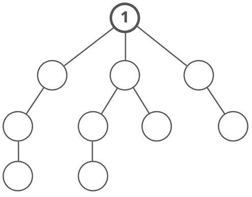
Breadth-first search (BFS) is a method for exploring a tree or graph. In a BFS, you first explore all the nodes one step away, then all the nodes two steps away, etc. Breadth-first search is like throwing a stone in the center of a pond. The nodes you explore "ripple out" from the starting point. Here's a how a BFS would traverse this tree, starting with the root:

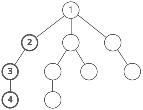
We'd visit all the immediate children (all the nodes that're one step away from our starting node):

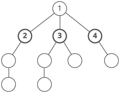
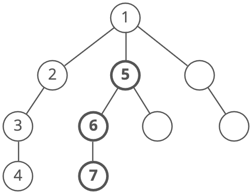
Then we'd move on to all those nodes' children (all the nodes that're two steps away from our starting node):

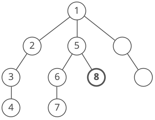
And so on:

Until we reach the end.

Breadth-first search is often compared with depth-first search.

Advantages:

• A BFS will find the shortest path between the starting point and any other reachable node. A depth-first search will not necessarily find the shortest path.

Disadvantages:

• A BFS on a binary tree generally requires more memory than a DFS.

Depth-First Search (DFS)

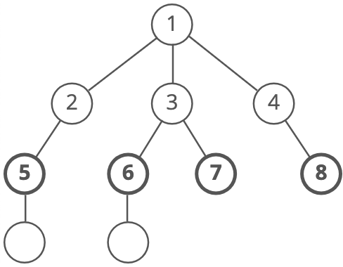
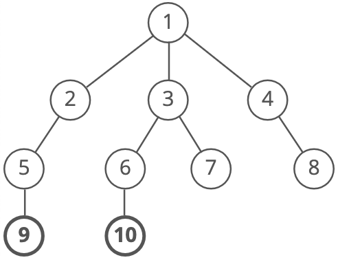
Depth-first search (DFS) is a method for exploring a tree or graph. In a DFS, you go as deep as possible down one path before backing up and trying a different one. Depth-first search is like walking through a corn maze. You explore one path, hit a dead end, and go back and try a different one.

Here's a how a DFS would traverse this tree, starting with the root:

We'd go down the first path we find until we hit a dead end:

Then we'd do the same thing again—go down a path until we hit a dead end:

And again:

And again:

Until we reach the end. Depth-first search is often compared with breadth-first search.

Advantages:

• Depth-first search on a binary tree generally requires less memory than breadth-first.
• Depth-first search can be easily implemented with recursion.

Disadvantages:

• A DFS doesn't necessarily find the shortest path to a node, while breadth-first search does.

Practice

Balanced Binary Tree

Write a function to see if a binary tree is "superbalanced" (a new tree property we just made up).

A tree is "superbalanced" if the difference between the depths of any two leaf nodes is no greater than one. (A leaf node is a tree node with no children. It's the "end" of a path to the bottom, from the root.)

Here's a sample binary tree node class:

class BinaryTreeNode(object):

    def __init__(self, value):
        self.value = value
        self.left  = None
        self.right = None

    def insert_left(self, value):
        self.left = BinaryTreeNode(value)
        return self.left

    def insert_right(self, value):
        self.right = BinaryTreeNode(value)
        return self.right

Hint 1

Sometimes it's good to start by rephrasing or "simplifying" the problem.

The requirement of "the difference between the depths of any two leaf nodes is no greater than 1" implies that we'll have to compare the depths of all possible pairs of leaves. That'd be expensive—-if there are $n$ leaves, there are $O(n^2)$ possible pairs of leaves.

But we can simplify this requirement to require less work. For example, we could equivalently say:

• "The difference between the min leaf depth and the max leaf depth is 1 or less"
• "There are at most two distinct leaf depths, and they are at most 1 apart"

Hint 2

If you're having trouble with a recursive approach, try using an iterative one.

Hint 3

To get to our leaves and measure their depths, we'll have to traverse the tree somehow. What methods do we know for traversing a tree?

Hint 4

Depth-first and breadth-first are common ways to traverse a tree. Which one should we use here?

Hint 5

The worst-case time and space costs of both are the same-—you could make a case for either.

But one characteristic of our algorithm is that it could short-circuit and return False as soon as it finds two leaves with depths more than 1 apart. So maybe we should use a traversal that will hit leaves as quickly as possible...

Hint 6

Depth-first traversal will generally hit leaves before breadth-first, so let's go with that. How could we write a depth-first walk that also keeps track of our depth?

Hint 7 (solution)

We do a depth-first walk through our tree, keeping track of the depth as we go. When we find a leaf, we add its depth to a list of depths if we haven't seen that depth already.

Each time we hit a leaf with a new depth, there are two ways that our tree might now be unbalanced:

1. There are more than 2 different leaf depths
2. There are exactly 2 leaf depths and they are more than 1 apart.

Why are we doing a depth-first walk and not a breadth-first one? You could make a case for either. We chose depth-first because it reaches leaves faster, which allows us to short-circuit earlier in some cases.

def is_balanced(tree_root):

    # A tree with no nodes is superbalanced, since there are no leaves!
    if tree_root is None:
        return True

    # We short-circuit as soon as we find more than 2
    depths = []

    # We'll treat this list as a stack that will store tuples of (node, depth)
    nodes = []
    nodes.append((tree_root, 0))

    while len(nodes):
        # Pop a node and its depth from the top of our stack
        node, depth = nodes.pop()

        # Case: we found a leaf
        if (not node.left) and (not node.right):
            # We only care if it's a new depth
            if depth not in depths:
                depths.append(depth)

                # Two ways we might now have an unbalanced tree:
                #   1) more than 2 different leaf depths
                #   2) 2 leaf depths that are more than 1 apart
                if ((len(depths) > 2) or
                        (len(depths) == 2 and abs(depths[0] - depths[1]) > 1)):
                    return False
        else:
            # Case: this isn't a leaf - keep stepping down
            if node.left:
                nodes.append((node.left, depth + 1))
            if node.right:
                nodes.append((node.right, depth + 1))

    return True

Complexity

$O(n)$ time and $O(n)$ space.

For time, the worst case is the tree is balanced and we have to iterate over all $n$ nodes to make sure.

For the space cost, we have two data structures to watch: depths and nodes.

depths will never hold more than three elements, so we can write that off as $O(1)$.

Because we're doing a depth first search, nodes will hold at most $d$ nodes where $d$ is the depth of the tree (the number of levels in the tree from the root node down to the lowest node). So we could say our space cost is $O(d)$.

But we can also relate $d$ to $n$. In a balanced tree, $d$ is $O(\log_2 n)$. And the more unbalanced the tree gets, the closer $d$ gets to $n$.

In the worst case, the tree is a straight line of right children from the root where every node in that line also has a left child. The traversal will walk down the line of right children, adding a new left child to nodes at each step. When the traversal hits the rightmost node, nodes will hold half of the $n$ total nodes in the tree. Half $n$ is $O(n)$, so our worst case space cost is $O(n)$.

What We Learned

This is an intro to some tree basics. If this is new to you, don't worry—-it can take a few questions for this stuff to come together. We have a few more coming up.

Particular things to note:

Focus on depth-first vs breadth-first traversal. You should be very comfortable with the differences between the two and the strengths and weaknesses of each.

You should also be very comfortable coding each of them up.

One tip: Remember that breadth-first uses a queue and depth-first uses a stack (could be the call stack or an actual stack object). That's not just a clue about implementation, it also helps with figuring out the differences in behavior. Those differences come from whether we visit nodes in the order we see them (first in, first out) or we visit the last-seen node first (last in, first out).

Binary Search Tree Checker

Write a function to check that a binary tree is a valid binary search tree.

Here's a sample binary tree node class:

class BinaryTreeNode(object):

    def __init__(self, value):
        self.value = value
        self.left  = None
        self.right = None

    def insert_left(self, value):
        self.left = BinaryTreeNode(value)
        return self.left

    def insert_right(self, value):
        self.right = BinaryTreeNode(value)
        return self.right

Hint 1

One way to break the problem down is to come up with a way to confirm that a single node is in a valid place relative to its ancestors. Then if every node passes this test, our whole tree is a valid BST.

Hint 2

What makes a given node "correct" relative to its ancestors in a BST? Two things:

• if a node is in the ancestor's left subtree, then it must be less than the ancestor, and
• if a node is in the ancestor's right subtree, then it must be greater than the ancestor.

Hint 3

So we could do a walk through our binary tree, keeping track of the ancestors for each node and whether the node should be greater than or less than each of them. If each of these greater-than or less-than relationships holds true for each node, our BST is valid.

The simplest ways to traverse the tree are depth-first and breadth-first. They have the same time cost (they each visit each node once). Depth-first traversal of a tree uses memory proportional to the depth of the tree, while breadth-first traversal uses memory proportional to the breadth of the tree (how many nodes there are on the "level" that has the most nodes).

Because the tree's breadth can as much as double each time it gets one level deeper, depth-first traversal is likely to be more space-efficient than breadth-first traversal, though they are strictly both $O(n)$ additional space in the worst case. The space savings are obvious if we know our binary tree is balanced—its depth will be $O(\lg n)$ and its breadth will be $O(n)$.

But we're not just storing the nodes themselves in memory, we're also storing the value from each ancestor and whether it should be less than or greater than the given node. Each node has $O(n)$ ancestors ($O(\lg n)$ for a balanced binary tree), so that gives us $O(n^2)$ additional memory cost ($O(n\lg n)$ for a balanced binary tree). We can do better.

Hint 4

Let's look at the inequalities we'd need to store for a given node:

Notice that we would end up testing that the blue node is <20, <30, and <50. Of course, <30 and <50 are implied by <20. So instead of storing each ancestor, we can just keep track of a lower_bound and upper_bound that our node's value must fit inside.

Hint 5 (solution)

Solution

We do a depth-first walk through the tree, testing each node for validity as we go. If a node appears in the left subtree of an ancestor, it must be less than that ancestor. If a node appears in the right subtree of an ancestor, it must be greater than that ancestor.

Instead of keeping track of every ancestor to check these inequalities, we just check the largest number it must be greater than (its lower_bound) and the smallest number it must be less than (its upper_bound).

def is_binary_search_tree(root):

    # Start at the root, with an arbitrarily low lower bound
    # and an arbitrarily high upper bound
    node_and_bounds_stack = [(root, -float('inf'), float('inf'))]

    # Depth-first traversal
    while len(node_and_bounds_stack):
        node, lower_bound, upper_bound = node_and_bounds_stack.pop()

        # If this node is invalid, we return false right away
        if (node.value <= lower_bound) or (node.value >= upper_bound):
            return False

        if node.left:
            # This node must be less than the current node
            node_and_bounds_stack.append((node.left, lower_bound, node.value))
        if node.right:
            # This node must be greater than the current node
            node_and_bounds_stack.append((node.right, node.value, upper_bound))

    # If none of the nodes were invalid, return true
    # (at this point we have checked all nodes)
    return True

Instead of allocating a stack ourselves, we could write a recursive function that uses the call stack. This would work, but it would be vulnerable to stack overflow. However, the code does end up quite a bit cleaner:

def is_binary_search_tree(root,
                          lower_bound=-float('inf'),
                          upper_bound=float('inf')):
    if not root:
        return True

    if (root.value >= upper_bound or root.value <= lower_bound):
        return False

    return (is_binary_search_tree(root.left, lower_bound, root.value)
            and is_binary_search_tree(root.right, root.value, upper_bound))

Checking if an in-order traversal of the tree is sorted is a great answer too, especially if you're able to implement it without storing a full list of nodes.

Complexity

$O(n)$ time and $O(n)$ space.

The time cost is easy: for valid binary search trees, we'll have to check all $n$ nodes.

Space is a little more complicated. Because we're doing a depth first search, node_and_bounds_stack will hold at most $d$ nodes where $d$ is the depth of the tree (the number of levels in the tree from the root node down to the lowest node). So we could say our space cost is $O(d)$.

But we can also relate $d$ to $n$. In a balanced tree, $d$ is $\log_2 n$. And the more unbalanced the tree gets, the closer $d$ gets to $n$.

In the worst case, the tree is a straight line of right children from the root where every node in that line also has a left child. The traversal will walk down the line of right children, adding a new left child to the stack at each step. When the traversal hits the rightmost node, the stack will hold half of the $n$ total nodes in the tree. Half $n$ is $O(n)$, so our worst case space cost is $O(n)$.

Bonus

What if the input tree has duplicate values?

What if -float('inf') or float('inf') appear in the input tree?

What We Learned

We could think of this as a greedy approach. We start off by trying to solve the problem in just one walk through the tree. So we ask ourselves what values we need to track in order to do that. Which leads us to our stack that tracks upper and lower bounds.

We could also think of this as a sort of "divide and conquer" approach. The idea in general behind divide and conquer is to break the problem down into two or more subproblems, solve them, and then use that solution to solve the original problem.

In this case, we're dividing the problem into subproblems by saying, "This tree is a valid binary search tree if the left subtree is valid and the right subtree is valid." This is more apparent in the recursive formulation of the answer above.

Of course, it's just fine that our approach could be thought of as greedy or could be thought of as divide and conquer. It can be both. The point here isn't to create strict categorizations so we can debate whether or not something "counts" as divide and conquer.

Instead, the point is to recognize the underlying patterns behind algorithms, so we can get better at thinking through problems.

Sometimes we'll have to kinda smoosh together two or more different patterns to get our answer.

2nd Largest Item in a Binary Search Tree

Write a function to find the 2nd largest element in a binary search tree.

Here's a sample binary tree node class:

class BinaryTreeNode(object):

    def __init__(self, value):
        self.value = value
        self.left  = None
        self.right = None

    def insert_left(self, value):
        self.left = BinaryTreeNode(value)
        return self.left

    def insert_right(self, value):
        self.right = BinaryTreeNode(value)
        return self.right

Hint 1

Let's start by solving a simplified version of the problem and see if we can adapt our approach from there. How would we find the largest element in a BST?

Hint 2

A reasonable guess is to say the largest element is simply the "rightmost" element.

So maybe we can start from the root and just step down right child pointers until we can't anymore (until the right child is null). At that point the current node is the largest in the whole tree.

Is this sufficient? We can prove it is by contradiction:

If the largest element were not the "rightmost," then the largest element would either:

1. be in some ancestor node's left subtree, or
2. have a right child.

But each of these leads to a contradiction:

1. If the node is in some ancestor node's left subtree it's smaller than that ancestor node, so it's not the largest.
2. If the node has a right child that child is larger than it, so it's not the largest.

So the "rightmost" element must be the largest.

How would we formalize getting the "rightmost" element in code?

Hint 3

We can use a simple recursive approach. At each step:

1. If there is a right child, that node and the subtree below it are all greater than the current node. So step down to this child and recurse.
2. Else there is no right child and we're already at the "rightmost" element, so we return its value.

def find_largest(root_node):

    if root_node.right:
        return find_largest(root_node.right)
    return root_node.value

Okay, so we can find the largest element. How can we adapt this approach to find the second largest element?

Hint 4

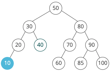
Our first thought might be, "it's simply the parent of the largest element!" That seems obviously true when we imagine a nicely balanced tree like this one:

.        ( 5 )
        /     \
      (3)     (8)
     /  \     /  \
   (1)  (4) (7)  (9)

But what if the largest element itself has a left subtree?

.        ( 5 )
        /     \
      (3)     (8)
     /  \     /  \
   (1)  (4) (7)  (12)
                 /
               (10)
               /  \
             (9)  (11)

Here the parent of our largest is 8, but the second largest is 11.

Drat, okay so the second largest isn't necessarily the parent of the largest...back to the drawing board...

Wait. No. The second largest is the parent of the largest if the largest does not have a left subtree. If we can handle the case where the largest does have a left subtree, we can handle all cases, and we have a solution.

So let's try sticking with this. How do we find the second largest when the largest has a left subtree?

Hint 5

It's the largest item in that left subtree! Whoa, we freaking just wrote a function for finding the largest element in a tree. We could use that here!

How would we code this up?

Hint 6

def find_largest(root_node):
    if root_node is None:
        raise ValueError('Tree must have at least 1 node')
    if root_node.right is not None:
        return find_largest(root_node.right)
    return root_node.value


def find_second_largest(root_node):
    if (root_node is None or
            (root_node.left is None and root_node.right is None)):
        raise ValueError('Tree must have at least 2 nodes')

    # Case: we're currently at largest, and largest has a left subtree,
    # so 2nd largest is largest in said subtree
    if root_node.left and not root_node.right:
        return find_largest(root_node.left)

    # Case: we're at parent of largest, and largest has no left subtree,
    # so 2nd largest must be current node
    if (root_node.right and
            not root_node.right.left and
            not root_node.right.right):
        return root_node.value

    # Otherwise: step right
    return find_second_largest(root_node.right)

Okay awesome. This'll work. It'll take $O(h)$ time (where $h$ is the height of the tree) and $O(h)$ space.

But that $h$ space in the call stack is avoidable. How can we get this down to constant space?

Hint 7 (solution)

We start with a function for getting the largest value. The largest value is simply the "rightmost" one, so we can get it in one walk down the tree by traversing rightward until we don't have a right child anymore:

def find_largest(root_node):

    current = root_node
    while current:
        if not current.right:
            return current.value
        current = current.right

With this in mind, we can also find the second largest in one walk down the tree. At each step, we have a few cases:

1. If we have a left subtree but not a right subtree, then the current node is the largest overall (the "rightmost") node. The second largest element must be the largest element in the left subtree. We use our find_largest() function above to find the largest in that left subtree!
2. If we have a right child, but that right child node doesn't have any children, then the right child must be the largest element and our current node must be the second largest element!
3. Else, we have a right subtree with more than one element, so the largest and second largest are somewhere in that subtree. So we step right.

def find_largest(root_node):
    current = root_node
    while current:
        if not current.right:
            return current.value
        current = current.right


def find_second_largest(root_node):
    if (root_node is None or
            (root_node.left is None and root_node.right is None)):
        raise ValueError('Tree must have at least 2 nodes')

    current = root_node
    while current:
        # Case: current is largest and has a left subtree
        # 2nd largest is the largest in that subtree
        if current.left and not current.right:
            return find_largest(current.left)

        # Case: current is parent of largest, and largest has no children,
        # so current is 2nd largest
        if (current.right and
                not current.right.left and
                not current.right.right):
            return current.value

        current = current.right

Complexity

We're doing one walk down our BST, which means $O(h)$ time, where $h$ is the height of the tree (again, that's $O(\lg n)$ if the tree is balanced, $O(n)$ otherwise). $O(1)$ space.

What We Learned

Here we used a "simplify, solve, and adapt" strategy.

The question asks for a function to find the second largest element in a BST, so we started off by simplifying the problem: we thought about how to find the first largest element.

Once we had a strategy for that, we adapted that strategy to work for finding the second largest element.

It may seem counter-intuitive to start off by solving the wrong question. But starting off with a simpler version of the problem is often much faster, because it's easier to wrap our heads around right away.

One more note about this one:

Breaking things down into cases is another strategy that really helped us here.

Notice how simple finding the second largest node got when we divided it into two cases:

1. The largest node has a left subtree.
2. The largest node does not have a left subtree.

Whenever a problem is starting to feel complicated, try breaking it down into cases.

It can be really helpful to actually draw out sample inputs for those cases. This'll keep your thinking organized and also help get your interviewer on the same page.

Graph Coloring

Note about induction proofs with graphs

In general, an inductive proof uses 2 steps to prove a claim is true for all (usually positive) integers:

1. A base case showing the claim is true for the first number (1 or 0)
2. An inductive step showing that if we assume the claim is true for a number $n$, then the claim is also true for $n+1$

If the claim is true for the first number, and for any next number, then it must be true for all numbers.

So let's prove this claim:

A legal coloring with $D+1$ colors is always possible for a graph of $N$ nodes with maximum degree $D$.

For our base case, we need to show this claim holds for a graph with 1 node.

A graph with 1 node has 0 edges, so the maximum degree $D$ is 0. That means we have 1 color ($D+1=1$).

Can we color that node with the one available color? Definitely, since it doesn't have any adjacent nodes that could make the coloring illegal.

What about if the graph has a loop! ↴ We're assuming our graph doesn't have these because otherwise, there's no possible legal coloring. Keep this edge case in mind though: we'll need to check for loops in our input graph and throw an error if we find any.

So we've proven our base case. Now for the inductive step.

This'll be our assumption:

A $D+1$ coloring is possible for a graph with $N$ nodes.

Can we show that if our assumption is true, it must also be true for a graph with $N+1$ nodes?

Let's say we have a graph with $N+1$ nodes and maximum degree $D$. We're not sure yet if we can color it with $D+1$ colors, right?

Ok, so let's remove a node and its edges from the graph. Any node. Now we have a graph with $N$ nodes.

What happened to $D$ by removing a node?

$D$ either stayed the same or went down. We removed edges, so there's no way $D$ went up.

So now we have a graph with $N$ nodes and maximum degree at most $D$. Can we color this graph with $D+1$ colors?

Yup! That's exactly our assumption! As part of the inductive step, we've assumed that we can color this graph with $D+1$ colors. So let's go ahead and color the graph.

Now all we have to do is add back in the node we removed (so we have $N+1$ nodes again) and show we can find a valid color for that node.

When we add the node we removed back in, what's the most neighbors it can have?

$D$. We started with a graph with $N+1$ nodes and maximum degree $D$, and we just rebuilt that graph.

In the worst case, the node we add back in will have $D$ neighbors, and they'll all have different colors. Not a problem. We have $D+1$ colors to choose from, so at least one color is still free. We'll use that one for this node. Bam.

Given an undirected graph with maximum degree $D$, find a graph coloring using at most $D+1$ colors.

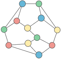
For example:

This graph's maximum degree ($D$) is 3, so we have 4 colors $(D+1)$. Here's one possible coloring:

Graphs are represented by a list of $N$ node objects, each with a label, a set of neighbors, and a color:

class GraphNode:

    def __init__(self, label):
        self.label = label
        self.neighbors = set()
        self.color = None


a = GraphNode('a')
b = GraphNode('b')
c = GraphNode('c')

a.neighbors.add(b)
b.neighbors.add(a)
b.neighbors.add(c)
c.neighbors.add(b)

graph = [a, b, c]

Hint 1

Let's take a step back. Is it always possible to find a legal coloring with $D+1$ colors?

Let's think about it. Each node has at most $D$ neighbors, and we have $D+1$ colors. So, if we look at any node, there's always at least one color that's not taken by its neighbors.

So yes—-$D+1$ is always enough colors for a legal coloring.

Still not convinced? We can prove this more formally using induction.

Okay, so there is always a legal coloring. Now, how can we find it?

Hint 2

A brute force approach would be to try every possible combination of colors until we find a legal coloring. Our steps would be:

1. For each possible graph coloring,
2. If the coloring is legal, then return it
3. Otherwise, move on to the next coloring

For example, looking back at our sample graph:

$D$ is 3, so we can use 4 colors. The combinations of 4 colors for all 12 nodes are:

red, red, red, red, red, red, red, red, red, red, red, red
red, red, red, red, red, red, red, red, red, red, red, yellow
red, red, red, red, red, red, red, red, red, red, red, green
red, red, red, red, red, red, red, red, red, red, red, blue
red, red, red, red, red, red, red, red, red, red, yellow, red
...
blue, blue, blue, blue, blue, blue, blue, blue, blue, blue, blue, green
blue, blue, blue, blue, blue, blue, blue, blue, blue, blue, blue, blue

And we'd keep trying combinations until we reach one that legally colors the graph.

This would work. But what's the complexity?

Here we'd try $4^{12}$ combinations (every combination of 4 colors for 12 nodes). In general, we'll have to check $O(D^N)$ colorings. And that's not all-—each time we try a coloring, we have to check all $M$ edges to see if the vertices at both ends have different colors. So, our runtime is $O(M\cdot D^N)$. That's exponential time since $N$ is in an exponent.

Since this algorithm is so inefficient, it's probably not what the interviewer is looking for. With practice, it gets easier to quickly judge if an approach will be inefficient. Still, sometimes it's a good idea in an interview to briefly explain inefficient ideas and why you think they're inefficient. It shows rigorous thinking.

How can we color the graph more efficiently?

Hint 3

Well, we're wasting a lot of time trying color combinations that don't work. If the first 2 nodes are neighbors, we shouldn't try any combinations where the first 2 colors are the same.

Hint 4

Instead of assigning all the colors at once, what if we colored the nodes one by one?

Hint 5

We could assign a color to the first node, then find a legal color for the second node, then for the third node, and keep going node by node.

def color_graph(graph, colors):
    for node in graph:
        # Get the node's neighbors' colors, as a set so we
        # can check if a color is illegal in constant time
        illegal_colors = set([
            neighbor.color
            for neighbor in node.neighbors
            if neighbor.color
        ])
        legal_colors = [
            color
            for color in colors
            if color not in illegal_colors
        ]

        # Assign the first legal color
        node.color = legal_colors[0]

Is it possible we'll back ourselves into a corner somehow and run out of colors for some nodes?

Let's think back to our earlier argument about whether a coloring always exists:

"Each node has at most $D$ neighbors, and we have $D+1$ colors. So, if we look at any node, there's always at least one color that's not taken by its neighbors."

That reasoning works here, too! So no-—we'll never back ourselves into a corner.

Ok, what's our runtime?

Hint 6

We're iterating through each node in the graph, so the loop body executes $N$ times. In each iteration of the loop:

1. We look at the current node's neighbors to figure out what colors are already taken. That's $O(D)$, since any given node can have up to $D$ neighbors.
2. Then, we look at all the colors (there are $O(D)$ of them) to see which ones are available.
3. Finally, we pick the first color that's free and assign it to the node ($O(1)$).

So our runtime is $N\cdot(D+D+1)$, which is $O(N\cdot D)$.

Can we tighten our analysis a bit here? Take a look at step 1, where we collect the neighbors' colors:

We said looking at each node's neighbors was $O(D)$ since each node can have at most $D$ neighbors ... but each node might have way fewer neighbors than that.

Can we say anything about the total number of neighbors we'll look at across all of the loop iterations? How many neighbors are there in the entire graph?

Each edge creates two neighbors: one for each node on either end. So when our code looks at every neighbor for every node, it looks at $2\cdot M$ neighbors in all. With $O(M)$ neighbors, collecting all the colors over the entire for loop takes $O(M)$ time.

Using this tighter analysis, we've taken our runtime from $N\cdot(D+D+1)$ down to $N\cdot(D+1)+M$. That's $O((N\cdot D)+M)$ time.

Of course, that complexity doesn't look any faster, at least not asymptotically. But in the underlying expression, we've gotten rid of one of the two $N\cdot D$ factors.

Can we get rid of the other one to bring our complexity down to linear time?

Hint 7

The remaining $N\cdot D$ factor comes from step 2: looking at every color for every node to populate legal_colors.

Do we have to look at every color for every node?

Hint 8

When we're coloring a node, we just need one color that hasn't been taken by any of the node's neighbors. We can stop looking at colors as soon as we find one:

def color_graph(graph, colors):
    for node in graph:
        # Get the node's neighbors' colors, as a set so we
        # can check if a color is illegal in constant time
        illegal_colors = set([
            neighbor.color
            for neighbor in node.neighbors
            if neighbor.color
        ])

        # Assign the first legal color
        for color in colors:
            if color not in illegal_colors:
                node.color = color
                break

Okay, now what's the time cost of assigning the first legal color to every node (the whole last block)?

We'll try at most len(illegal_colors) + 1 colors in total. That's how many we'd need if we happen to test all the colors in illegal_colors first, before finally testing the one legal color last.

Remember the "+1" we get from testing the one legal color last! It's going to be important in a second.

How many colors are in illegal_colors? It's at most the number of neighbors, if each neighbor has a different color.

Let's use that trick of looking at all of the loop iterations together. In total, over the course of the entire loop, how many neighbors are there?

Well, each of our $M$ edges adds two neighbors to the graph: one for each node on either end. So that's $2\cdot M$ neighbors in total. Which means $2\cdot M$ illegal colors in total.

But remember: we said we'd try as many as len(illegal_colors) + 1 colors per node. We still have to factor in that "+1"! Across all $N$ of our nodes, that's an additional $N$ colors. So we try $2\cdot M+N$ colors in total across all of our nodes.

That's $O(M+N)$ time for assigning the first legal color to every node. Add that to the $O(M)$ for finding all the illegal colors, and we get $O(M+N)$ time in total for our graph coloring function.

Is this the fastest runtime we can get? We'll have to look at every node ($O(N)$) and every edge ($O(M)$) at least once, so yeah, we can't get any better than $O(N+M)$.

How about our space cost?

The only data structure we allocate with non-constant space is the set of illegal colors. What's the most space that ever takes up?

In the worst case, the neighbors of the node with the maximum degree will all have different colors, so our space cost is $O(D)$.

Before we're done, what about edge cases?

Hint 9

For graph problems in general, edge cases are:

• nodes with no edges
• cycles
• loops

What if there are nodes with no edges? Will our function still color every node?

Hint 10

Yup, no problem. Isolated nodes tend to cause problems when we're traversing a graph (starting from one node and "walking along" edges to other nodes, like we do in a depth-first or breadth-first search). We're not doing that here—-instead, we're iterating over a list of all the nodes.

What if the graph has a cycle? Will our function still work?

Hint 11

Yes, it will. Cycles also tend to cause problems with graph traversal, because we can end up in infinite loops (going around and around the cycle). But we're not actually traversing our graph here.

What if the graph has a loop?

Hint 12

That's a problem. A node with a loop is adjacent to itself, so it can't have the same color as ... itself. So it's impossible to "legally color" a node with a loop. So we should throw an error.

How can we detect loops?

Hint 13

We know a node has a loop if the node is in its own set of neighbors.

Hint 14 (solution)

Solution

We go through the nodes in one pass, assigning each node the first legal color we find.

How can we be sure we'll always have at least one legal color for every node? In a graph with maximum degree $D$, each node has at most $D$ neighbors. That means there are at most $D$ colors taken by a node's neighbors. And we have $D+1$ colors, so there's always at least one color left to use.

When we color each node, we're careful to stop iterating over colors as soon as we find a legal color.

def color_graph(graph, colors):
    for node in graph:
        if node in node.neighbors:
            raise Exception('Legal coloring impossible for node with loop: %s' %
                            node.label)

        # Get the node's neighbors' colors, as a set so we
        # can check if a color is illegal in constant time
        illegal_colors = set([
            neighbor.color
            for neighbor in node.neighbors
            if neighbor.color
        ])

        # Assign the first legal color
        for color in colors:
            if color not in illegal_colors:
                node.color = color
                break

Complexity

$O(N+M)$ time where $N$ is the number of nodes and $M$ is the number of edges.

The runtime might not look linear because we have outer and inner loops. The trick is to look at each step and think of things in terms of the total number of edges ($M$) wherever we can:

• We check if each node appears in its own set of neighbors. Checking if something is in a set is $O(1)$, so doing it for all $N$ nodes is $O(N)$.
• When we get the illegal colors for each node, we iterate through that node's neighbors. So in total, we cross each of the graphs $M$ edges twice: once for the node on either end of each edge. $O(M)$ time.
• When we assign a color to each node, we're careful to stop checking colors as soon as we find one that works. In the worst case, we'll have to check one more color than the total number of neighbors. Again, each edge in the graph adds two neighbors—-one for the node on either end—-so there are $2\cdot M$ neighbors. So, in total, we'll have to try $O(N+M)$ colors.

Putting all the steps together, our complexity is $O(N+M)$.

What about space complexity? The only thing we're storing is the illegal_colors set. In the worst case, all the neighbors of a node with the maximum degree ($D$) have different colors, so our set takes up $O(D)$ space.

Bonus

1. Our solution runs in $O(N+M)$ time but takes $O(D)$ space. Can we get down to $O(1)$ space?
2. Our solution finds a legal coloring, but there are usually many legal colorings. What if we wanted to optimize a coloring to use as few colors as possible?

The lowest number of colors we can use to legally color a graph is called the chromatic number.

There's no known polynomial time solution for finding a graph's chromatic number. It might be impossible, or maybe we just haven't figured out a solution yet.

We can't even determine in polynomial time if a graph can be colored using a given $k$ colors. Even if $k$ is as low as 3.

We care about polynomial time solutions ($n$ raised to a constant power, like $O(n^2)$ because for large $n$s, polynomial time algorithms are more practical to actually use than higher runtimes like exponential time (a constant raised to the power of $n$, like $O(2^n)$. Computer scientists usually call algorithms with polynomial time solutions feasible, and problems with worse runtimes intractable.

The problem of determining if a graph can be colored with $k$ colors is in the class of problems called NP (nondeterministic polynomial time). This means that in polynomial time, we can verify a solution is correct but we can't come up with a solution. In this case, if we have a graph that's already colored with $k$ colors we verify the coloring uses $k$ colors and is legal, but we can't take a graph and a number $k$ and determine if the graph can be colored with $k$ colors.

If you can find a solution or prove a solution doesn't exist, you'll win a $1,000,000 Millennium Problem Prize.

For coloring a graph using as few colors as possible, we don't have a feasible solution. For real-world problems, we'd often need to check so many possibilities that we'll never be able to use brute-force no matter how advanced our computers become.

One way to reliably reduce the number of colors we use is to use the greedy algorithm but carefully order the nodes. For example, we can prioritize nodes based on their degree, the number of colored neighbors they have, or the number of uniquely colored neighbors they have.

What We Learned

We used a greedy approach to build up a correct solution in one pass through the nodes.

This brought us close to the optimal runtime, but we also had to take that last step of iterating over the colors only until we find a legal color. Sometimes stopping a loop like that is just a premature optimization that doesn't bring down the final runtime, but here it actually made our runtime linear!

MeshMessage

You wrote a trendy new messaging app, MeshMessage, to get around flaky cell phone coverage.

Instead of routing texts through cell towers, your app sends messages via the phones of nearby users, passing each message along from one phone to the next until it reaches the intended recipient. (Don't worry—-the messages are encrypted while they're in transit.)

Some friends have been using your service, and they're complaining that it takes a long time for messages to get delivered. After some preliminary debugging, you suspect messages might not be taking the most direct route from the sender to the recipient.

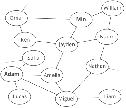
Given information about active users on the network, find the shortest route for a message from one user (the sender) to another (the recipient). Return a list of users that make up this route.

There might be a few shortest delivery routes, all with the same length. For now, let's just return any shortest route.

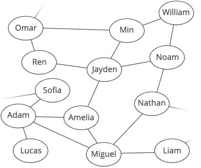
Your network information takes the form of an object where keys are usernames and values are lists of other users nearby:

network = {
    'Min'     : ['William', 'Jayden', 'Omar'],
    'William' : ['Min', 'Noam'],
    'Jayden'  : ['Min', 'Amelia', 'Ren', 'Noam'],
    'Ren'     : ['Jayden', 'Omar'],
    'Amelia'  : ['Jayden', 'Adam', 'Miguel'],
    'Adam'    : ['Amelia', 'Miguel', 'Sofia', 'Lucas'],
    'Miguel'  : ['Amelia', 'Adam', 'Liam', 'Nathan'],
    'Noam'    : ['Nathan', 'Jayden', 'William'],
    'Omar'    : ['Ren', 'Min', 'Scott'],
    ...
}

For the network above, a message from Jayden to Adam should have this route:

['Jayden', 'Amelia', 'Adam']

Hint 1

Users? Connections? Routes? What data structures can we build out of that? Let's run through some common ones and see if anything fits here.

• lists? Nope-—those are a bit too simple to express our network of users.
• Dictionaries? Maybeee.
• Graphs? Yeah, that seems like it could work!

Let's run with graphs for a bit and see how things go. Users will be nodes in our graph, and we'll draw edges between users who are close enough to message each other.

Our input object already represents the graph we want in adjacency list format. Each key in the object is a node, and the associated value-—a list of connected nodes—-is an adjacency list.

Is our graph directed or undirected? Weighted or unweighted?

Hint 2

For directed vs. undirected, we'll assume that if Min can transmit a message to Jayden, then Jayden can also transmit a message to Min. Our sample input definitely suggests this is the case. And it makes sense-—they're the same distance from each other, after all. That means our graph is undirected.

What about weighted? We're not given any information suggesting that some transmissions are more expensive than others, so let's say our graph is unweighted.

These assumptions seem pretty reasonable, so we'll go with them here. But, this is a great place to step back and check in with your interviewer to make sure they agree with what you've decided so far.

Here's what our user network looks like as a graph:

Okay, how do we start looking around our graph to find the shortest route from one user to another?

Or, more generally, how do we find the shortest path from a start node to an end node in an unweighted, undirected graph?

Hint 3

There are two common ways to explore undirected graphs: depth-first search (DFS) and breadth-first search (BFS).

Which do we want here?

Hint 4

Since we're interested in finding the shortest path, BFS is the way to go.

Remember: both BFS and DFS will eventually find a path if one exists. The difference between the two is:

• BFS always finds the shortest path.
• DFS usually uses less space.

Okay, so let's do a breadth-first search of our graph starting from the sender and stopping when we find the recipient. Since we're using breadth-first search, we know that the first time we see the recipient, we'll have traveled to them along the shortest path.

To code this up, let's start with a standard implementation of breadth-first search:

It's a good idea to know breadth-first and depth-first search well enough to quickly write them out. They show up in a lot of graph problems.

from collections import deque

def bfs(graph, start_node, end_node):
    nodes_to_visit = deque()
    nodes_to_visit.append(start_node)

    # Keep track of what nodes we've already seen
    # so we don't process them twice
    nodes_already_seen = set([start_node])

    while len(nodes_to_visit) > 0:
        current_node = nodes_to_visit.popleft()

        # Stop when we reach the end node
        if current_node == end_node:
            # Found it!
            break

        for neighbor in graph[current_node]:
            if neighbor not in nodes_already_seen:
                nodes_already_seen.add(neighbor)
                nodes_to_visit.append(neighbor)

Look at the nodes_already_seen set—-that's really important and easy to forget. If we didn't have it, our algorithm would be slower (since we'd be revisiting tons of nodes) and it might never finish (if there's no path to the end node).

We're using a queue instead of a list because we want an efficient first-in-first-out (FIFO) structure with $O(1)$ inserts and removes. If we used a list, appending would be $O(1)$, but removing elements from the front would be $O(n)$.

This seems like we're on the right track: we're doing a breadth-first search, which gets us from the start node to the end node along the shortest path.

But we're still missing an important piece: we didn't actually store our path anywhere. We need to reconstruct the path we took. How do we do that?

Well, we know that the first node in the path is start_node. And the next node in the path is ... well ... hmm.

Maybe we can start from the end and work backward? We know that the last node in the path is end_node. And the node before that is ... hmm.

We don't have enough information to actually reconstruct the path.

What additional information can we store to help us?

Hint 5

Well, to reconstruct our path, we'll need to somehow recover how we found each node. When do we find new nodes?

We find new nodes when iterating through current_node's neighbors.

So, each time we find a new node, let's jot down what current_node was when we found it. Like this:

from collections import deque

def bfs_get_path(graph, start_node, end_node):
    nodes_to_visit = deque()
    nodes_to_visit.append(start_node)

    # Keep track of what nodes we've already seen
    # so we don't process them twice
    nodes_already_seen = set([start_node])

    # Keep track of how we got to each node
    # we'll use this to reconstruct the shortest path at the end
    how_we_reached_nodes = {start_node: None}

    while len(nodes_to_visit) > 0:
        current_node = nodes_to_visit.popleft()

        # Stop when we reach the end node
        if current_node == end_node:
            # Somehow reconstruct the path here
            return path

        for neighbor in graph[current_node]:
            if neighbor not in nodes_already_seen:
                nodes_already_seen.add(neighbor)
                nodes_to_visit.append(neighbor)
                # Keep track of how we got to this node
                how_we_reached_nodes[neighbor] = current_node

Great. Now we just have to take that bookkeeping and use it to reconstruct our path! How do we do that?

Hint 6

Let's start by looking up start_node in our dictionary. Oops, it's just None.

Oh. Right. Our dictionary tells us which node comes before a given node on the shortest path. And nothing comes before the start node.

What about the end_node? If we look up the end node in how_we_reached_nodes, we'll get the node we were visiting when we found end_node. That's the node that comes right before the end node along the shortest path!

So, we'll actually be building our path backward from end_node to start_node.

Going back to our example, to recover the shortest path from Min to Adam:

We'd take this dictionary we built up during our search:

{
  'Min'     : None,
  'Jayden'  : 'Min',
  'Ren'     : 'Jayden',
  'Amelia'  : 'Jayden',
  'Adam'    : 'Amelia',
  'Miguel'  : 'Amelia',
  'William' : 'Min'
}

And, we'd use it to backtrack from the end node to the start node, recovering our path:

• To get to Adam, we went through Amelia.
• To get to Amelia, we went through Jayden.
• To get to Jayden, we went through Min.
• Min is the start node.

Chaining this together, the shortest path from Min to Adam is

Here's what this could look like in code:

def reconstruct_path(how_we_reached_nodes, start_node, end_node):
    shortest_path = []

    # Start from the end of the path and work backwards
    current_node = end_node

    while current_node:
        shortest_path.append(current_node)
        current_node = how_we_reached_nodes[current_node]

    return shortest_path

One small thing though. Won't this return a path that has the recipient at the beginning?

Oh. Since we started our backtracking at the recipient's node, our path is going to come out backward. So, let's reverse it before returning it:

shortest_path.reverse()  # now from start_node to end_node
return shortest_path  # return in the right order

Okay. That'll work!

But, before we're done, let's think about edge cases and optimizations.

What are our edge cases, and how should we handle them?

Hint 7

What happens if there isn't a route from the sender to the recipient?

If that happens, then we'll finish searching the graph without ever reconstructing and returning the path. That's a valid outcome—-it just means we can't deliver the message right now. So, if we finish our search and haven't returned yet, let's return None to indicate that no path was found.

What about if either the sender or recipient aren't in our user network?

That's invalid input, so we should throw an exception.

Any other edge cases?

Those two should be it. So, let's talk about optimizations. Can we make our algorithm run faster or take less space?

Hint 8

One thing that stands out is that we have two data structures—-nodes_already_seen and how_we_reached_nodes—-that are updated in similar ways. In fact, every time we add a node to nodes_already_seen, we also add it to how_we_reached_nodes. Do we need both of them?

We definitely need how_we_reached_nodes in order to reconstruct our path. What about nodes_already_seen?

Every node that appears in nodes_already_seen also appears in our object. So, instead of keeping a separate set tracking nodes we've already seen, we can just use the keys in how_we_reached_nodes. This lets us get rid of nodes_already_seen, which saves us $O(n)$ space.

Hint 9 (solution)

Solution

We treat the input user network as a graph in adjacency list ↴ format. Then we do a breadth-first search from the sender, stopping once we reach the recipient.

In order to recover the actual shortest path from the sender to the recipient, we do two things:

1. during our breadth-first search, we keep track of how we reached each node, and
2. after our breadth-first search reaches the end node, we use our object to backtrack from the recipient to the sender.

To make sure our breadth-first search terminates, we're careful to avoid visiting any node twice. We could keep track of the nodes we've already seen in a set, but, to save space, we reuse the object we've already set up for recovering the path.

from collections import deque


def reconstruct_path(previous_nodes, start_node, end_node):
    reversed_shortest_path = []

    # Start from the end of the path and work backwards
    current_node = end_node
    while current_node:
        reversed_shortest_path.append(current_node)
        current_node = previous_nodes[current_node]

    # Reverse our path to get the right order
    reversed_shortest_path.reverse()  # flip it around, in place
    return reversed_shortest_path  # no longer reversed


def bfs_get_path(graph, start_node, end_node):
    if start_node not in graph:
        raise Exception('Start node not in graph')
    if end_node not in graph:
        raise Exception('End node not in graph')

    nodes_to_visit = deque()
    nodes_to_visit.append(start_node)

    # Keep track of how we got to each node
    # We'll use this to reconstruct the shortest path at the end
    # We'll ALSO use this to keep track of which nodes we've
    # already visited
    how_we_reached_nodes = {start_node: None}

    while len(nodes_to_visit) > 0:
        current_node = nodes_to_visit.popleft()

        # Stop when we reach the end node
        if current_node == end_node:
            return reconstruct_path(how_we_reached_nodes, start_node, end_node)

        for neighbor in graph[current_node]:
            if neighbor not in how_we_reached_nodes:
                nodes_to_visit.append(neighbor)
                how_we_reached_nodes[neighbor] = current_node

    # If we get here, then we never found the end node
    # so there's NO path from start_node to end_node
    return None

Complexity

Our solution has two main steps. First, we do a breadth-first search of the user network starting from the sender. Then, we use the results of our search to backtrack and find the shortest path.

How much work is a breadth-first search?

In the worst case, we'll go through the BFS loop once for every node in the graph, since we only ever add each node to nodes_to_visit once (we check how_we_reached_nodes to see if we've already added a node before). Each loop iteration involves a constant amount of work to dequeue the node and check if it's our end node. If we have $n$ nodes, then this portion of the loop is $O(N)$.

But there's more to each loop iteration: we also look at the current node's neighbors. Over all of the nodes in the graph, checking the neighbors is $O(M)$, since it involves crossing each edge twice: once for each node at either end.

Putting this together, the complexity of the breadth-first search is $O(N+M)$.

BFS and DFS are common enough that it's often acceptable to just state their complexity as $O(N+M)$. Some interviewers might want you to derive it though, so definitely be ready in case they ask.

What about backtracking to determine the shortest path? Handling each node in the path is $O(1)$, and we could have at most $N$ nodes in our shortest path. So, that's $O(N)$ for building up the path. Then, it's another $O(N)$ to reverse it. So, the total time complexity of our backtracking step is $O(N)$.

Putting these together, the time complexity of our entire algorithm is $O(N+M)$.

What about space complexity? The queue of nodes to visit, the mapping of nodes to previous nodes, and the final path ... they all store a constant amount of information per node. So, each data structure could take up to $O(N)$ space if it stored information about all of our nodes. That means our overall space complexity is $O(N)$.

Bonus

1. In our solution, we assumed that if one user (Min) could transmit a message to another (Jayden), then Jayden would also be able to transmit a message to Min. Suppose this wasn't guaranteed—maybe Min's cell phone transmits over shorter distances than Jayden's. How would our graph change to represent this? Could we still use BFS?
2. What if we wanted to find the shortest path? Assume we're given a GPS location for each user. How could we incorporate the distance between users into our graph? How would our algorithm change?
3. In our solution, we assumed that users never moved around. How could we extend our algorithm to handle the graph changing over time?

Our app's design has a formal name: a mesh network. In a mesh network, data is sent from one node (here, a phone) to another directly, rather than through intermediate devices (here, cell towers). Assuming enough devices are in range, mesh networks provide multiple possible transmission paths, making them reliable even if some devices have failed.

What We Learned

The tricky part was backtracking to assemble the path we used to reach our end_node. In general, it's helpful to think of backtracking as two steps:

1. Figuring out what additional information we need to store in order to rebuild our path at the end (how_we_reached_nodes, in this case).
2. Figuring out how to reconstruct the path from that information.

And in this case, something interesting happened after we added how_we_reached_nodes-—it made nodes_already_seen redundant! So we were able to remove it. A good reminder to always look through your variables at the end and see if there are any you can cut out.

Find Repeat, Space Edition BEAST MODE

In Find a duplicate, Space Edition™, we were given a list of integers where:

1. the integers are in the range $1\ldots n$
2. the list has a length of $n+1$

These properties mean the list must have at least 1 duplicate. Our challenge was to find a duplicate number without modifying the input and optimizing for space. We used a divide and conquer approach, iteratively cutting the list in half to find a duplicate integer in $O(n\lg n)$ time and $O(1)$ space (sort of a modified binary search).

But we can actually do better. We can find a duplicate integer in $O(n)$ time while keeping our space cost at $O(1)$.

This is a tricky one to derive (unless you have a strong background in graph theory), so we'll get you started:

Imagine each item in the list as a node in a linked list. In any linked list, each node has a value and a "next" pointer. In this case:

• The value is the integer from the list.
• The "next" pointer points to the value-eth node in the list (numbered starting from 1). For example, if our value was 3, the "next" node would be the third node.

Here's a full example:

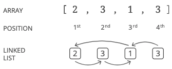
Notice we're using "positions" and not "indices." For this problem, we'll use the word "position" to mean something like "index," but different: indices start at 0, while positions start at 1. More rigorously: position = index + 1.

Using this, find a duplicate integer in $O(n)$ time while keeping our space cost at $O(1)$. Just like before, don't modify the input.

Drawing pictures will help a lot with this one. Grab some paper and pencil (or a whiteboard, if you have one).

Hint 1

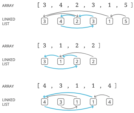
Here are a few sample lists. Try drawing them out as linked lists:

[3, 4, 2, 3, 1, 5]
[3, 1, 2, 2]
[4, 3, 1, 1, 4]

Look for patterns. Then think about how we might use those patterns to find a duplicate number in our list.

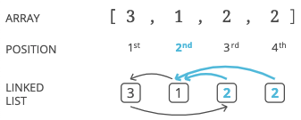
Hint 2

When a value is repeated, how will that affect the structure of our linked list?

Hint 3

If two nodes have the same value, their next pointers will point to the same node!

So if we can find a node with two incoming next pointers, we know the position of that node is a duplicate integer in our list.

For example, if there are two 2s in our list, the node in the 2nd position will have two incoming pointers.

Alright, we're on to something. But hold on-—creating a linked list would take $O(n)$ space, and we don't want to change our space cost from $O(1)$.

No problem—-turns out we can just think of the list as a linked list, and traverse it without actually creating a new data structure.

If you're stuck on figuring out how to traverse the list like a linked list, don't sweat it too much. Just use a real linked list for now, while we finish deriving the algorithm.

Ok, so we figured out that the position of a node with multiple incoming pointers must be a duplicate. If we can find a node with multiple incoming pointers in a constant number of walks through our list, we can find a duplicate value in $O(n)$ time.

How can we find a node with multiple incoming pointers?

Hint 4

Let's look back at those sample lists and their corresponding linked lists, which we drew out to look for patterns:

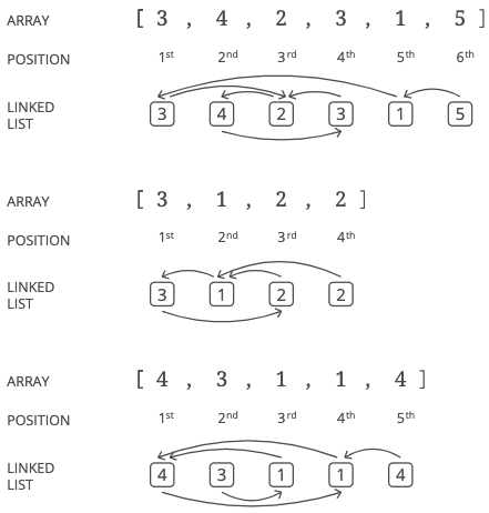
Are there any patterns that might help us find a node with two incoming pointers?

Hint 5

Here's a pattern: the last node never has any incoming pointers. This makes sense—-since the list has a length $n+1$ and all the values are $n$ or less, there can never be a pointer to the last position. If $n$ is 5, the length of the list is 6 but there can't be a value 6 so no pointer will ever point to the 6th node. Since it has no incoming pointers, we should treat the last position in our list as the "head" (starting point) of our linked list.

Here's another pattern: there's never an end to our list. No pointer ever points to null. Every node has a value in the range $1\ldots n$, so every node points to another node (or to itself). Since the list goes on forever, it must have a cycle (a loop). Here are the cycles in our example lists:

Can we use these cycles to find a duplicate value?

Hint 6

If we walk through our linked list, starting from the head, at some point we will enter our cycle. Try tracing that path on the example lists above. Notice anything special about the first node we hit when we enter the cycle?

Hint 7

The first node in the cycle always has at least two incoming pointers!

Hint 8

We're getting close to an algorithm for finding a duplicate value. How can we find the beginning of a cycle?

Hint 9

Again, drawing an example is helpful here:

If we were traversing this list and wanted to know if we were inside a cycle, that would be pretty easy-—we could just remember our current position and keep stepping ahead to see if we get to that position again.

But our problem is a little trickier—-we need to know the first node in the cycle.

What if we knew the length of the cycle?

Hint 10

If we knew the length of the cycle, we could use the "stick approach" to start at the head of the list and find the first node. We use two pointers. One pointer starts at the head of the list:

Then we lay down a "stick" with the same length as the cycle, by starting the second pointer at the end. So here, for example, the second pointer is starting 4 steps ahead because the cycle has 4 steps:

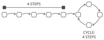
Then we move the stick along the list by advancing the two pointers at the same speed (one node at a time).

When the first pointer reaches the first node in the cycle, the second pointer will have circled around exactly once. The stick wraps around the cycle, and the two ends are in the same place: the start of the cycle.

We already know where the head of our list is (the last position in the list) so we just need the length of the cycle. How can we find the length of a cycle?

Hint 11

If we can get inside the cycle, we can just remember a position and count how many steps it takes to get back to that position.

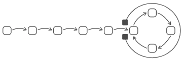
How can we make sure we've gotten inside a cycle?

Hint 12

Well, there has to be a cycle in our list, and at the latest, the cycle is just the last node we hit as we traverse the list from the head:

So we can just start at the head and walk $n$ steps. By then we'll have to be inside a cycle.

Hint 13

Alright, we've pieced together an entire strategy to find a duplicate integer! Working backward:

1. We know the position of a node with multiple incoming pointers is a duplicate in our list because the nodes that pointed to it must have the same value.
2. We find a node with multiple incoming pointers by finding the first node in a cycle.
3. We find the first node in a cycle by finding the length of the cycle and advancing two pointers: one starting at the head of the linked list, and the other starting ahead as many steps as there are steps in the cycle. The pointers will meet at the first node in the cycle.
4. We find the length of a cycle by remembering a position inside the cycle and counting the number of steps it takes to get back to that position.
5. We get inside a cycle by starting at the head and walking $n$ steps. We know the head of the list is at position $n+1$.

Can you implement this? And remember—-we won't want to actually create a linked list. Here's how we can traverse our list as if it were a linked list.

Elaboration

Let's take an example list and try walking through it as if it were a linked list:

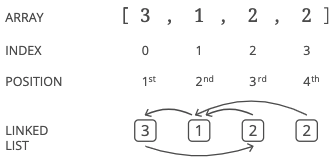
Remember that our input list is defined as having a length $n+1$. So we know $n$ is 3 because the list has a length of 4.

The head (starting point) is the 4th node, since it has no incoming pointers. We'll want to go from the 4th position to the 2nd position to the 1st position to the 3rd position. Or, in terms of indices in our list, we'll want to go from index 3 to index 1 to index 0 to index 2.

Let's get set up:

n = 3
int_list = [3, 1, 2, 2]

# start at the head
current_position = 4

Now we need to take $n$ steps:

for _ in range(n):
    # step ahead

On our first step, current_position is 4 and the value at the 4th position is 2, so we want to update current_position to 2. The only trick is that we need to convert our position to an index. That's easy—-we just subtract 1 (the 1st position of a list is index 0).

for _ in range(n):

    # subtract 1 from the current position to get
    # the current index
    current_index = current_position - 1

    # take a step, updating the current position
    # to the *value* at its previous position
    current_position = int_list[current_index]

So if welre at a current_position, the next position we want to go to is the value at the index current_position - 1. We can refactor this to 1 line and have this general way to take $n$ steps forward in our list as if it were a linked list:

for _ in range(number_of_steps):
    current_position = int_list[current_position - 1]

Hint 14

To get inside a cycle (step 5 above), we identify $n$, start at the head (the node in position $n+1$), and walk $n$ steps.

def find_duplicate(int_list):
    n = len(int_list) - 1

    # STEP 1: GET INSIDE A CYCLE
    # Start at position n+1 and walk n steps to
    # find a position guaranteed to be in a cycle
    position_in_cycle = n + 1
    for _ in range(n):
        position_in_cycle = int_list[position_in_cycle - 1]

Hint 15

Now we're guaranteed to be inside a cycle. To find the cycle's length (D), we remember the current position and step ahead until we come back to that same position, counting the number of steps.

def find_duplicate(int_list):
    n = len(int_list) - 1

    # STEP 1: GET INSIDE A CYCLE
    # Start at position n+1 and walk n steps to
    # find a position guaranteed to be in a cycle
    position_in_cycle = n + 1
    for _ in range(n):
        position_in_cycle = int_list[position_in_cycle - 1]

    # STEP 2: FIND THE LENGTH OF THE CYCLE
    # Find the length of the cycle by remembering a position in the cycle
    # and counting the steps it takes to get back to that position
    remembered_position_in_cycle = position_in_cycle
    current_position_in_cycle = int_list[position_in_cycle - 1]  # 1 step ahead
    cycle_step_count = 1

    while current_position_in_cycle != remembered_position_in_cycle:
        current_position_in_cycle = int_list[current_position_in_cycle - 1]
        cycle_step_count += 1

Hint 16

Now we have the head and the length of the cycle. We need to find the first node in the cycle (C). We set up 2 pointers: 1 at the head, and 1 ahead as many steps as there are nodes in the cycle. These two pointers form our "stick."

# STEP 3: FIND THE FIRST NODE OF THE CYCLE
# Start two pointers
#   (1) at position n+1
#   (2) ahead of position n+1 as many steps as the cycle's length
pointer_start = n + 1
pointer_ahead = n + 1
for _ in range(cycle_step_count):
    pointer_ahead = int_list[pointer_ahead - 1]

Hint 17

Alright, we just need to find to the first node in the cycle (B), and return a duplicate value (A)!

Hint 18 (solution)

We treat the input list as a linked list like we described at the top in the problem.

To find a duplicate integer:

1. We know the position of a node with multiple incoming pointers is a duplicate in our list because the nodes that pointed to it must have the same value.
2. We find a node with multiple incoming pointers by finding the first node in a cycle.
3. We find the first node in a cycle by finding the length of the cycle and advancing two pointers: one starting at the head of the linked list, and the other starting ahead as many steps as there are nodes in the cycle. The pointers will meet at the first node in the cycle.
4. We find the length of a cycle by remembering a position inside the cycle and counting the number of steps it takes to get back to that position.
5. We get inside a cycle by starting at the head and walking $n$ steps. We know the head of the list is at position $n+1$.

We want to think of our list as a linked list but we don't want to actually use up all that space, so we traverse our list as if it were a linked list by converting positions to indices.

def find_duplicate(int_list):
    n = len(int_list) - 1

    # STEP 1: GET INSIDE A CYCLE
    # Start at position n+1 and walk n steps to
    # find a position guaranteed to be in a cycle
    position_in_cycle = n + 1
    for _ in range(n):
        position_in_cycle = int_list[position_in_cycle - 1]
        # we subtract 1 from the current position to step ahead:
        # the 2nd *position* in a list is *index* 1

    # STEP 2: FIND THE LENGTH OF THE CYCLE
    # Find the length of the cycle by remembering a position in the cycle
    # and counting the steps it takes to get back to that position
    remembered_position_in_cycle = position_in_cycle
    current_position_in_cycle = int_list[position_in_cycle - 1]  # 1 step ahead
    cycle_step_count = 1

    while current_position_in_cycle != remembered_position_in_cycle:
        current_position_in_cycle = int_list[current_position_in_cycle - 1]
        cycle_step_count += 1

    # STEP 3: FIND THE FIRST NODE OF THE CYCLE
    # Start two pointers
    #   (1) at position n+1
    #   (2) ahead of position n+1 as many steps as the cycle's length
    pointer_start = n + 1
    pointer_ahead = n + 1
    for _ in range(cycle_step_count):
        pointer_ahead = int_list[pointer_ahead - 1]

    # Advance until the pointers are in the same position
    # which is the first node in the cycle
    while pointer_start != pointer_ahead:
        pointer_start = int_list[pointer_start - 1]
        pointer_ahead = int_list[pointer_ahead - 1]

    # Since there are multiple values pointing to the first node
    # in the cycle, its position is a duplicate in our list
    return pointer_start

Complexity

$O(n)$ time and $O(1)$ space.

Our space cost is $O(1)$ because all of our additional variables are integers, which each take constant space.

For our runtime, we iterate over the list a constant number of times, and each iteration takes $O(n)$ time in its worst case. So we traverse the linked list more than once, but it's still a constant number of times—-about 3.

Bonus

There another approach using randomized algorithms that is $O(n)$ time and $O(1)$ space. Can you come up with that one? (Hint: You'll want to focus on the median.)

What We Learned

This one's pretty crazy. It's hard to imagine an interviewer expecting you to get all the way through this question without help.

But just because it takes a few hints to get to the answer doesn't mean a question is "too hard." Some interviewers expect they'll have to offer a few hints.

So if you get a hint in an interview, just relax and listen. The most impressive thing you can do is drop what you're doing, fully understand the hint, and then run with it.